PyTorch with the MNIST Dataset
PyTorch is a open-source library that takes the machine learning tools of Torch and adapts them for use in Python. The following code is adopted from the PyTorch examples repository. It is licensed under BSD 3-Clause “New” or “Revised” License.
This notebook uses the following pedagogical patterns:
Learning Objectives
- Learn how to utilize PyTorch
- Employ Pytorch in the creation of an image-recognition algorithm
Problem Definition
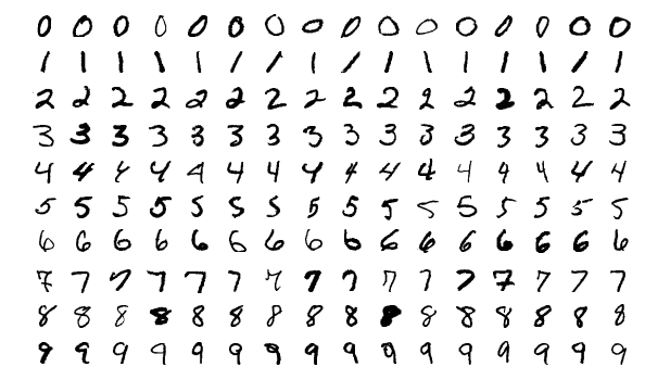
To illustrate the computational power of PyTorch, we will take a crack at processing the MNIST database. MNIST is a database of 70,000 images of handwritten numbers used to evaluate image processing techniques. From Kaggle:
MNIST (“Modified National Institute of Standards and Technology”) is the de facto “hello world” dataset of computer vision. Since its release in 1999, this classic dataset of handwritten images has served as the basis for benchmarking classification algorithms. As new machine learning techniques emerge, MNIST remains a reliable resource for researchers and learners alike.
Check out this table from Wikipedia to see what kind of machine learning methods generate good error rates.
PyTorch vs. Tensorflow
PyTorch serves as a great tool for learning data science because of its flexibility when compared to other libraries. Below are a few points of comparison between PyTorch and another popular dataflow tool, Tensorflow:
- PyTorch enables dynamic computational graphs, while Tensorflow’s computation is static. This means that at runtime PyTorch defines the graph’s structure, which can be changed depending on parameters like the input data. Conversely, Tensorflow needs to have the structure defined before running.
- Tensorflow enables easier deployment and requires less memory because it only has to worry about computations at the end.
Setting up PyTorch
Start by installing PyTorch with the following command:
!pip install torch torchvision
We will then import all of the libraries needed for our algorithm.
from __future__ import print_function
import argparse
import torch
import torch.nn as nn
import torch.nn.functional as F
import torch.optim as optim
from torchvision import datasets, transforms
from torch.autograd import Variable
Next we can define the arguments for our functions and then load in our data.
args={}
kwargs={}
args['batch_size']=1000
args['test_batch_size']=1000
args['epochs']=10     #The number of Epochs is the number of times you go through the full dataset.
args['lr']=0.01       #Learning rate is how fast it will decend.
args['momentum']=0.5  #SGD momentum (default: 0.5) Momentum is a moving average of our gradients (helps to keep direction).

args['seed']=1        #random seed
args['log_interval']=10
args['cuda']=False
#load the data
train_loader = torch.utils.data.DataLoader(
    datasets.MNIST('../data', train=True, download=True,
                   transform=transforms.Compose([
                       transforms.ToTensor(),
                       transforms.Normalize((0.1307,), (0.3081,))
                   ])),
    batch_size=args['batch_size'], shuffle=True, **kwargs)
test_loader = torch.utils.data.DataLoader(
    datasets.MNIST('../data', train=False, transform=transforms.Compose([
                       transforms.ToTensor(),
                       transforms.Normalize((0.1307,), (0.3081,))
                   ])),
    batch_size=args['test_batch_size'], shuffle=True, **kwargs)
class Net(nn.Module):
    #This defines the structure of the NN.
    def __init__(self):
        super(Net, self).__init__()
        self.conv1 = nn.Conv2d(1, 10, kernel_size=5)
        self.conv2 = nn.Conv2d(10, 20, kernel_size=5)
        self.conv2_drop = nn.Dropout2d()  #Dropout
        self.fc1 = nn.Linear(320, 50)
        self.fc2 = nn.Linear(50, 10)

    def forward(self, x):
        #Convolutional Layer/Pooling Layer/Activation
        x = F.relu(F.max_pool2d(self.conv1(x), 2))
        #Convolutional Layer/Dropout/Pooling Layer/Activation
        x = F.relu(F.max_pool2d(self.conv2_drop(self.conv2(x)), 2))
        x = x.view(-1, 320)
        #Fully Connected Layer/Activation
        x = F.relu(self.fc1(x))
        x = F.dropout(x, training=self.training)
        #Fully Connected Layer/Activation
        x = self.fc2(x)
        #Softmax gets probabilities.
        return F.log_softmax(x, dim=1)
def train(epoch):
    model.train()
    for batch_idx, (data, target) in enumerate(train_loader):
        if args['cuda']:
            data, target = data.cuda(), target.cuda()
        #Variables in Pytorch are differenciable.
        data, target = Variable(data), Variable(target)
        #This will zero out the gradients for this batch.
        optimizer.zero_grad()
        output = model(data)
        # Calculate the negative log likelihood loss - it's useful to train a classification problem with C classes.
        loss = F.nll_loss(output, target)
        #dloss/dx for every Variable
        loss.backward()
        #to do a one-step update on our parameter.
        optimizer.step()
        #Print out the loss periodically.
        if batch_idx % args['log_interval'] == 0:
            print('Train Epoch: {} [{}/{} ({:.0f}%)]\tLoss: {:.6f}'.format(
                epoch, batch_idx * len(data), len(train_loader.dataset),
                100. * batch_idx / len(train_loader), loss.data[0]))

def test():
    model.eval()
    test_loss = 0
    correct = 0
    for data, target in test_loader:
        if args['cuda']:
            data, target = data.cuda(), target.cuda()
        data, target = Variable(data, volatile=True), Variable(target)
        output = model(data)
        test_loss += F.nll_loss(output, target, size_average=False).data[0] # sum up batch loss
        pred = output.data.max(1, keepdim=True)[1] # get the index of the max log-probability
        correct += pred.eq(target.data.view_as(pred)).long().cpu().sum()

    test_loss /= len(test_loader.dataset)
    print('\nTest set: Average loss: {:.4f}, Accuracy: {}/{} ({:.0f}%)\n'.format(
        test_loss, correct, len(test_loader.dataset),
        100. * correct / len(test_loader.dataset)))
model = Net()
if args['cuda']:
    model.cuda()

optimizer = optim.SGD(model.parameters(), lr=args['lr'], momentum=args['momentum'])

for epoch in range(1, args['epochs'] + 1):
    train(epoch)
    test()

